Excel CTRL Key Tricks

Excel CTRL Key Tricks

Table of Contents

ctrl key tricks

The Excel CTRL key tricks. That dull, grey-beige looking key that lives an unassuming, lonely life on the edge of your keyboard actually leads an exciting double life in Excel. Now, this is not going to be a life changing experience for you but it may bring a touch of fun into otherwise unexciting everyday tasks. Read on.

Copying and Moving Worksheet Cells

Cut and Paste is most peoples’s favourite method of moving data from one cell to another. A simpler alternative is Drag and Drop; point to any of the cell’s borders, wait for the arrow pointer to display and then drag your data to another cell.

If you want to drag your selection onto another worksheet, drag down to the sheet tabs and then hold down the ALT key to switch over to the other worksheet.
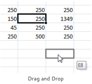
drag and drop
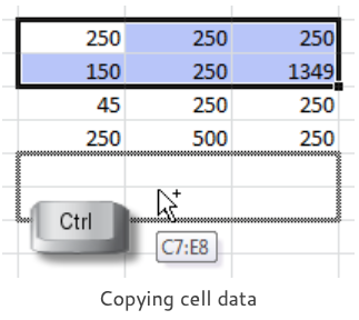
copying cell data

To change your move into a copy (Copy and Paste), hold down the CTRL key as you drag. You should see that a plus sign is displayed next to the arrow pointer. Keep your CTRL key held down until you have released the mouse button.

Cell drag and drop is usually enabled. Should you find that the arrow pointer does not display then you need to turn it on. The settings is in Excel Options (File tab), Advanced section, Editing options: Enable fill handle and cell drag-and-drop.

Copying and Moving Columns and Rows

Drag and Drop works in exactly the same way for moving or copying entire columns or rows. Just click the column letter or row number first to select it and then point to the edge of the selection. Drag to move or CTRL+Drag to copy.
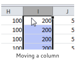
moving a column

Copying and Moving Worksheets

You’ve already figured it out; the drag and drop method is equally effective for copying and moving entire worksheets. Point to the sheet tab and click, the document icon will display. Now drag to the left or right hand side to move the worksheet into a new position in the workbook.
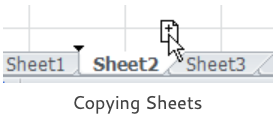
To make a copy of an entire worksheet, point to the sheet tab and click. When the document icon displays, hold down the CTRL key and you will see a plus sign displayed on the icon. Now, drag the sheet to the left or right hand side to create a copy. Try doing that with Copy and Paste.
 
On some keyboards you need to hold down the CTRL first before clicking the sheet tab.
 
copying sheets
a copied sheet
arrange all

If your worksheets are in different workbooks then you can still drag and drop your worksheets but you need to have both of the workbooks visible first. Arrange the documents on the screen by clicking the View tab,  then go to the Window group and click Arrange All, Tiled.  Drag to move a worksheet, CTRL+Drag to copy.
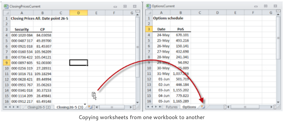
copying worksheets from one workbook to another

Drag and Drop with the Shift Key

Don’t forget the SHIFT key. When you drag and drop one cell onto another you usually overwrite the data in the destination cell or range of cells.

But when you hold down the SHIFT key as you drag then you insert cells into the destination range without overwriting data.
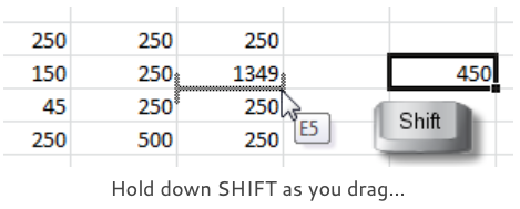
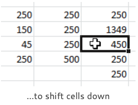
hold down shift as you drag
to shift cells down

Watch the I-beam as you drag, the vertical I-beam means Shift cells right and the horizontal I-beam means Shift cells down.

In the illustrations we took the 450 cell value over to the right and dragged it into the E5 cell position and the rest of the cell range moved down to accommodate the data insertion.

Filling Data with the Fill handle

The Fill handle is that little black cross-shaped mouse pointer that appears at the lower right corner of the active cell. Not unreasonably, it is popularly known as the “little black cross”. When you drag the Fill handle down or across you fill the data from the active cell across or down: formulas are copied, numbers are copied as constants and text stored in an Custom list, such as days of the week, triggers the list sequence.

When you hold down the CTRL key as you drag you will see a plus sign displayed on the black cross and this reverses the normal behaviour of the fill. For example, if you drag a cell containing the value of 1 then the number 1 will remain constant but if you hold down the CTRL key then you will generate the sequence of values: 1,2,3,4 etc.
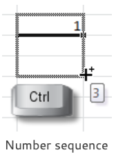
number sequence
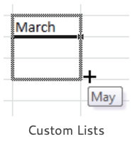
custom lists

Normal text is copied as a constant but Custom list text is entered in the order of the custom list. Custom lists can be very handy; for example you type “March” into a cell then you drag to enter the other months of the year.

But this can be irritating if you wish the month name to remain constant. This is where you hold down the CTRL key to reverse the usual action. Type in “March” and then CTRL+Drag to copy “March” into the cells below.

Excel Custom lists can be viewed, edited and set up in Options (File tab), Advanced section, scroll down to General and click the Edit Custom Lists control.

Repeating Patterns with the Fill handle

Sequences of numbers may be generated by creating a seed pattern in a few cells and then selecting this seed pattern and dragging to extend the sequence. For example a plus 10 sequence is seeded by typing 10 and 20 into consecutive cells, then you select the two cells and drag to generate the sequence 10,20,30,40,50 etc.

Repetitions of the seed pattern are obtained by holding down the CTRL key as you drag. The sequence of values is then repeated; 10,20,10,20,10,20 etc.
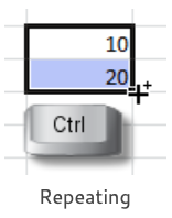
repeating cell data

Making Multiple Selections

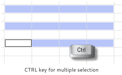
A multiple selection of cells is where you select one range of cells and then you hold down the CTRL key and keep it held down as you continue to add to your initial selection and create a collection.
 
If you make a mistake then there’s nothing to be done other than to click a cell to clear your current selection and start over again.
 
This sort of selection is so useful for cell formatting as you can apply your formats to the entire selection in one fell swoop instead of having to format each range individually and invaluable where you want to plot cell ranges which are not immediately adjacent to each other on an Excel chart.
ctrl key for multiple selection
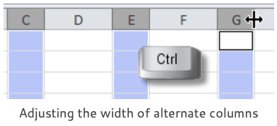
adjusting width of alternate columns

The same method of selection is easily applied to entire columns or rows by clicking the first column letter or row number, then you hold down the CTRL key and click on the others.

With multiple rows selected you can apply actions such as deletion to all the selected rows or with multiple columns selected, as in the illustration, you can change the width of alternate columns in your worksheet. The more you use collections the more ideas you will have. Not all actions can be applied to a multiple selection but it is always worth experimenting.

Now we’ve got the general idea. In the illustration below we coloured alternate sheet tabs red in one go by holding down the CTRL key and clicking on the relevant sheet tabs. Right-click any selected tab to access the Tab Color command.

colouring alternate sheet tabs

And the Shift Key again…

The other method of selection that is useful to know is Block selection which uses the SHIFT key. This is the selection of a continuous range of cells effected not by dragging, as is usual, but by clicking. You click the first cell of your selection, hold down the SHIFT key and then click the last cell. It’s Click, Shift, Click.

This feels very awkward if you never tried it before as you can not stop yourself from dragging but if you practice the technique on small ranges of cells then you will rapidly master it. And then you can apply in so many different situations: selecting huge ranges of cells, ranges of sheet tabs etc.
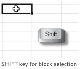
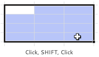
shift key for block selection
click, shift, click

Now you’re an expert in the dark art of Excel cell selection you will find that you can use these selection techniques on other Excel objects and in other Microsoft Office applications. 

Extend Mode

A final word on multiple selection, using your keyboard. The CTRL key with a normal mouse is the easiest thing in the world, you hold the key down with your left hand and select with your right hand. But left-handers don’t always have such an easy time of it and some touch pads can make you wish that you had a third hand. This is where you need Extend Mode with the keyboard.

Press function key F8 to open extend mode and then select your first cell range either using your mouse or by using your keyboard: hold down the SHIFT key and extend the selection by pressing your arrow keys.
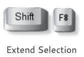
extend selection

Now, lock your current selection by pressing SHIFT+F8 and then move on to make your next selection. This is best done by pressing the arrow keys to exit the current selection and then pressing SHIFT and arrow keys again to make the next selection. Press SHIFT+F8 again to lock this selection and continue in this way until the selection is complete.

I can assure you that this is a lot easier to do than it is to read about it.

Related Courses

Microsoft Excel Introduction – Link

Microsoft Excel Intermediate – Link

Excel Drop Down Lists

Excel Drop Down Lists

Table of Contents

Excel drop down lists

There are three different types of Excel drop down lists available:

  1. “Pick from” lists which are generated automatically.
  2. Data Validation lists which are very easy to do.
  3. Combo box and List box controls which require a bit more work.

Pick from lists

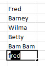
As you type a list of data into a column in your worksheet you are automatically prompted with previously entered list elements that match your typed characters. In the illustration, I have typed in an “f” and the cell is filled-in with “fred” as this entry is already in the list.
 
To accept the prompted text, press ENTER or press the Down Arrow key. To decline the suggestion, keep typing.
pick from list
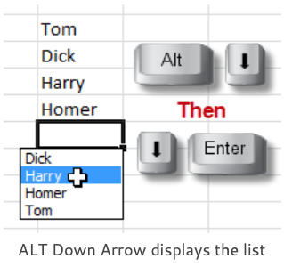
ALT down arrow displays the list
To generate the list entries without your having to do any initial typing, you can use the shortcut key combination ALT + Down Arrow to display the list elements and then, if you’re a keyboard fan, press the Down Arrow key again to go down through the list and then ENTER to accept the entry.
 
If you can’t be bothered with all this good old-fashioned shortcut keys business then just right-click in the cell and choose Pick from Drop-down list in the shortcut menu.
 

Data Validation lists

These lists are used where you want to restrict the entry made in a cell to only those items available in a drop-down list. The list of valid entries can be typed in or you can refer to a range of cells which contains your valid entries.  The range of valid entries can be entered into a different worksheet in the same workbook.

data validation control
data validation

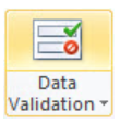
Data Validation lists are ideal not only where you need to make sure that people make the right entry but also for data entry generally as it is so easy to choose from a drop-down list. To create the validation list, select the cell or range of cells where you want the list to be displayed and then click the Data Validation control on the Data tab (look for Data Validation in the Data menu if you are using an older version of Excel)

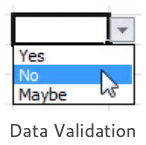
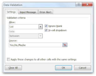
In the Settings tab, choose List from the Allow drop-down list and then type in a comma-separated list of your valid entries into the Source box. In this case, the list items are Yes, No and Maybe. Click the OK button and you’re done. The list is available when you click on one of the cells where the validation has been applied and data entry into the cell is restricted to only those items in the list. 

Click the Error Alert tab if you want to change the standard “the value you entered is not valid” error message for invalid entries. You may prefer something a little more personal. 

data validation dialog

Using a range of cells to provide the source

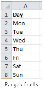
A range of cells is preferable for your data validation where you either have a long list or you want to be able to change the list regularly.

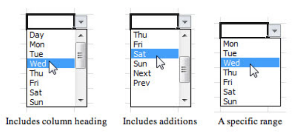
You can set the Source data validation as either a horizontal or vertical range of cells or an entire column or row. Either type in the range reference or (far easier) select the range or click the column letter or row number.

When you click the column letter remember that any heading at the top of your list on the worksheet will be included as the first item in your validation list. But if you add to the list on the worksheet then these additional items will automatically appear in the validation list. So there are advantages and disadvantages to selecting the whole column.

If you specify a range of cells then then you don’t have the headings issue to deal with but if you then add to the list on the worksheet then you will also have to remember to reset the Source data range to include your additions.

range of cells
types of drop down

Displaying the drop-down list in alphabetical order

The drop-down list is linked to the values in the worksheet cells, so sort the list in the cells in alphabetical order if you wish to show the drop-down list in the same order. But you can’t have the drop-down list in a different order.

Dependant Data Validation lists

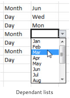
Sometimes you need the choice that you have made in one list to control the list shown in another cell; one of your validation lists is dependant on the other.

In the illustration there are two columns, the first column shows the class of date required, “Month” or “Day”. This is entered from a simple comma separated validation list which is typed in. The second column needs to show either a list of months if “Month” is entered in the corresponding cell in the first column or a list of days if “Day” is entered.

There are two ranges of cells in the worksheet named as Month and Day respectively which are going to be the alternative source ranges for the second column (see the next section if you are not sure how to Name a range) When you set the source data range for the second column enter the following formula: =INDIRECT(A2)

dependant lists

Where A2 is the first cell in the first column where you have your “Day” or “Month” entry. Of course, you should change this cell reference to suit your own worksheet. The INDIRECT function is well named as it makes the reference indirect, i.e. not A2 but the range reference entered in A2. In other words, if it’s “Day” then show the Day list, if it’s “Month” then show the Month list. You’re not restricted to just having a choice between two alternative lists, with this method you can have the choice of as many different lists as you like.

If this does not seem to work for you then try checking the following points:

  1. Did you select the area for the dependant range before applying the Data Validation? In the example above it would have been the second column. It’s very easy to apply validation to a single cell when you intended to set it for a range.
  2. Check the spelling of the range names (in this case “Day” and “Month”) in the first list. They must be spelled correctly and you have to remember them as you type them in as comma separated values.
  3. Did you remember to name the ranges?

Naming a Range

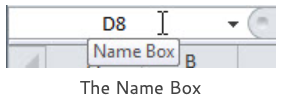
If you’re not sure how to name a range of cells then I would recommend using the Name Box, which is that area on the extreme left-hand side of the formula bar where you normally see your active cell reference. It’s not the only way of naming a range but most people find it to be the easiest way.

name box
name the range

Type in the name (in this example it is “Months”) and then press the ENTER key to register the name correctly. Please don’t click out of the box after typing the name, press ENTER. Sorry for being boring but that’s where it’s so easy to go wrong. Click the drop-down arrow to check that the name is available.

Combo box and List box controls

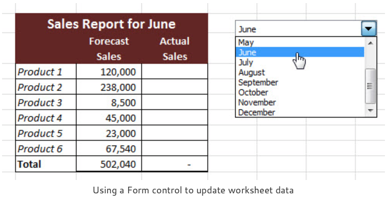
These are interactive graphics which are drawn on top of the worksheet cells and are then linked to certain key worksheet cells. They are commonly employed as a user-friendly graphical device to make user-unfriendly processes involving formulas much easier to control. 
form control to update worksheet data

In the above example, there is a combo box control containing a list of months. When a month is selected from the list the heading in the worksheet report is updated (“Sales Report for …”) and the relevant monthly numbers are extracted from another worksheet where the full twelve month’s Forecast Sales figures are entered.

All this is done by using Excel formulas but you don’t need to know anything about the formulas to use the worksheet. You just choose a month from the drop down list. Combo box and List box controls are quite easy to do, the hard bit is doing all the formulas.

Form controls

There are two sets of graphical controls available in Excel, Form controls and ActiveX controls. They both do much the same job but in rather different ways so it doesn’t matter which set you use.
 
Form controls were designed and built for Excel, ActiveX controls are more general controls used in many different applications. Form controls are simple and robust whereas ActiveX controls are more sophisticated and the process of using them takes far longer. It’s a judgement call. I shall be using Form controls in this example and deal with ActiveX in a future article.

Finding the Form controls

This is the first job. Form controls are not openly available, you need to display the Developer tab on your Excel ribbon. Click the File tab and then click Options. Click Customize Ribbon and then click the Developer check box in the Main Tabs list on the right-hand side. Click OK. Form controls are in the Insert control on the Controls group of the Developer tab.

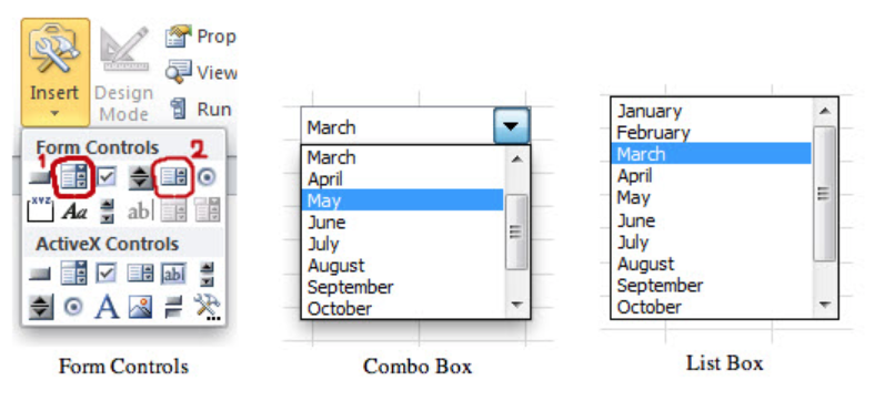
combo box and list box

Click the Insert control, the Form Controls are the top group. The Combo Box (1) control is the second one in from the left. The List box (2) control is second in from the right. Both controls behave the same; the Combo box is a drop-down list, the List box is an open list.

Creating the Combo Box

You need to go through a few steps to get the Combo box working. Firstly, create some cell ranges where you are going to store the data that you want to have displayed in the drop-down list and a cell to link the Combo box to. When you format your Combo box these ranges are going to be your Input range and your Cell link.

Personally, I would always put these data ranges on a separate worksheet so that I can then hide it. In the example I shall be using Named Ranges, as they are so easy to work with, rather than normal cell references but this is just personal preference. Use Named Ranges or the standard A1-style cell references as you prefer, they both work fine.
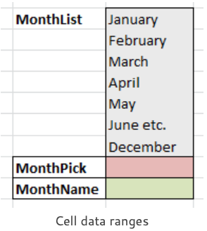
cell data ranges

In the illustration, I have a list of my twelve months (shortened for clarity) these are the grey cells and are named MonthList. The pink cell is going to be the cell link and is named MonthPick and the green cell is MonthName, where I am going to enter a formula which will calculate the current month. Now it’s time to create the Combo box, there’s three steps:

  1. Draw and format the Combo box
  2. Set the Input Range and Cell Link
  3. Test the Combo box and the enter the formulas
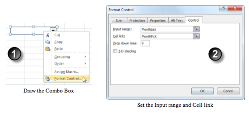
form controls combo box
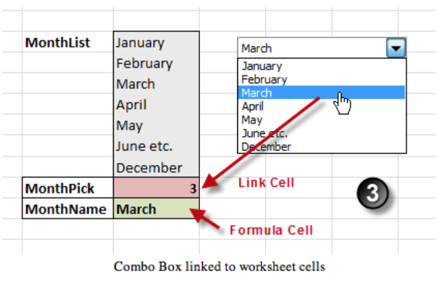
combo box linked to worksheet cells
  1. Draw the Combo box. Click the Combo box control and then drag to draw a horizontal rectangular shape. You can resize it later if it’s not quite right. Right-click the control to display its shortcut menu. Try to right-click when your mouse pointer is pointing to the middle of the control as there are different shortcut menus available, you want the one that contains Format Control.
  2. Format the Combo box. In the Format Control dialog enter the Input Range (in this example MonthList) and the Cell link (MonthPick) Click OK.
  3. Test the Combo box. Click a worksheet cell to take the focus away from the Combo box. It’s now active. Click the drop-down arrow and choose an item from the list. You should see that a value is returned into your link cell. It’s an index value, it’s not the text from the list. If you choose “March” from the list then the index is the value of 3 because it’s the third item in the list.

That’s the Combo box control completed and now it’s time to enter our formulas in the worksheet to make everything happen.

Entering the formulas

When you choose a month from the list you want to trigger the following processes in your formulas:

  1. Update the month name definition. This formula goes in the cell named MonthName so that we can use the name in our formulas wherever we need the selected month declared.
  2. Update the report heading with the name of the month.
  3. Update the report by showing the relevant data for the selected month.

1. Formula in the MonthName cell

Use the index value MonthPick to return the relevant item from the MonthList list using Excel’s INDEX function. The formula is:

=INDEX(MonthList,MonthPick)

2. Update the report heading with the name of the month

The named range MonthName updates to show the currently selected month so we concatenate it’s value with the static text “Sales Report for …”. This formula is entered on the worksheet where we have our report. The formula is:

=”Sales Report for “&MonthName

3. Update the Sales Forecast figures to show the currently selected month

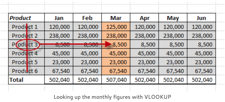
There’s various ways of doing this but the most obvious way is to use the index value MonthPick in a Lookup formula to return the current month’s figures from the range containing all the year’s Sales Forecast figures.

looking up monthly figures with VLOOKUP
In the illustration above, the grey cells are named SalesForecast. This range is on a different worksheet but that’s not a problem when we use a named range. When the selected month from the Combo box is “March” then the value of MonthPick is 3. The corresponding “March” figures are in the 4th column of the SalesForecast range so if we add the value of 1 to MonthPick then we calculate the correct column index value for our lookup formula. The formula is:
 
=VLOOKUP(B5, SalesForecast, MonthPick+1, FALSE)
 
Where B5 is the cell reference of the first Product in the main report (it contains the text “Product 1”), SalesForecast is the lookup range, MonthPick+1 the column index value and FALSE because it is an Exact Match VLOOKUP based on matching the product name in the main report to the products listed in the first column of the lookup range.

Related Courses

Microsoft Excel Intermediate – Link

Microsoft Excel Advanced – Link

Excel AutoSum Revisited

Excel AutoSum Revisited

Table of Contents

autosum control

Excel AutoSum Revisited

You just can’t get away from AutoSum. If I had a pound for every time I’ve clicked AutoSum to add up a column of numbers I would probably be sitting on a tropical island somewhere still clicking it to add up all my vast wealth. It’s one of the first things you learn about in Excel and, of course, everybody knows it inside out.

Column and Row Totals

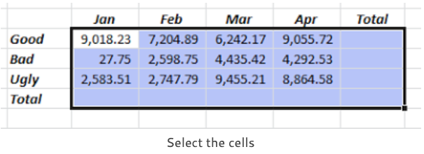
Here’s a really easy way of calculating column and row totals without having to do all that infernal copying. The first job is to select all the cells containing your numbers and extend the selection to the empty cells where you want the totals.

select the cells
click autosum

Then you click AutoSum and you’re done! It really is that easy. If you only want the column totals then just select the cells with the numbers and the totals are returned into the row below.

Here’s all the column and row totals done in two simple steps. And they are done perfectly as the range references in the SUMs are implied by the selection. They hardly need to be checked.

column and row totals

If you prefer to do the whole thing with your keyboard then hold down the SHIFT key and extend the cell selection by pressing the arrow keys. Then use the shortcut key combination ALT= to generate the SUM formulas.

autosum shortcut

Grand Totals

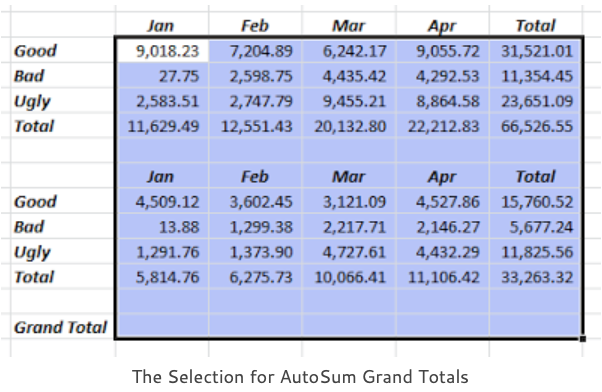
But it’s not just one table is it, you’ve got loads of them and some serious number crunching to do. You can extend the select-and-click-AutoSum method to do grand totals as well. But, be careful, this method only really works if every line item in your worksheet is drawn into a subtotal.
selection for autosum grand totals
Firstly, calculate all of your individual subtotals and then make a selection of all of the cells containing your numbers and the cells containing your subtotals.
 
Now, click AutoSum and all the cells containing your subtotal SUMs are detected and the Grand Total is calculated correctly without any risk of double-counting.
 
Here’s the resulting formulas displayed in the cells and you clearly see the formulas containing the original range references for the subtotal SUMs.

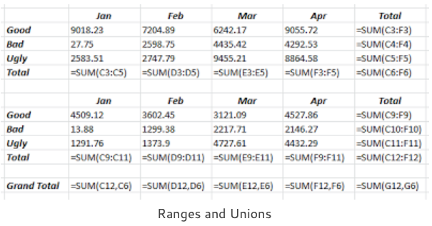
All the grand total SUMs generated by AutoSum are Unions, showing each subtotal reference separated by commas. Number-crunching never has been much fun but this certainly better than having to construct Grand Totals from plus signs and cell references.

Our SUM formulas usually contain Range References, using a colon separator. For example, C3:C5 means “from C3 to C5”. Union references use commas. For example, C12, C16 means C12 and C16.

ranges and unions

Checking your Formulas

As some of us know from bitter experience it is very embarrassing when a simple mistake in your formulas messes up all your careful calculations. So, it’s always a good policy to check that you’ve got your formulas right but it’s a bit painful to view them individually in the formula bar.

show the formulas

You can display the formulas directly in the cells by clicking the Show Formulas control. It’s in the Formula Auditing group of the Formulas tab. Click once to show the formulas and click again to show the results.

formulas displayed in the cells
If you have a really old version of Excel then you have to search in the Tools, Options dialog for this option which is not much fun and I recommend that you use the shortcut key combination CTRL ` (that’s usually the key under the ESC key on the top right of your keyboard) Press the keys once to display the formulas and again to show the returned results.
Show formulas shortcut

Related Courses

Microsoft Excel Intermediate – Link

Microsoft Excel Advanced – Link

Excel Top Ten Shortcut Keys

Excel Top Ten Shortcut Keys

Table of Contents

excel top ten shortcut keys

Excel Top Ten Shortcut Keys

Ask ten people what their favourite Excel shortcut keys are and you’ll get ten different answers. In no particular order, here’s my personal choice of the ones that I can’t do without. I’m not going to list ALL the Excel shortcut keys here because there are hundreds of them.


Ctrl+A  Select the Current Region

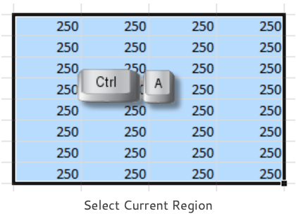
Click a cell, press Ctrl+A and Excel expands your selection to select the Current Region. Press Ctrl+A again and the entire worksheet is selected.

The Current Region is defined as the current area of continuous data bounded by blank cells. In older versions of Excel you may have to press the key combination Ctrl+* to achieve the same effect (Ctrl+SHIFT+* if you don’t have a dedicated *key)

select current region

Ctrl+Spacebar  Select the Current Column

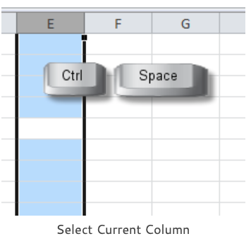
What, pick up my mouse and click the column letter. No way! Ctrl+Spacebar selects your current column and then to extend the selection to the left or right you hold down the SHIFT key and use the Left or Right arrow key

select current column

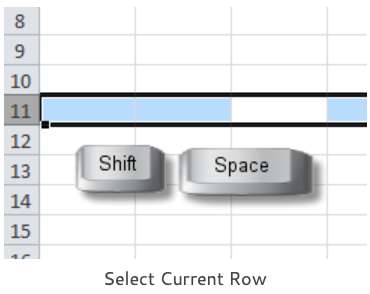
SHIFT+Spacebar Select the Current Row

Well, I did say that it’s a personal choice. Lazy-bones here selects the current row with SHIFT+Spacebar. Then keep the SHIFT key held down and press the Up or Down arrow keys to extend the selection up or down.

select current row

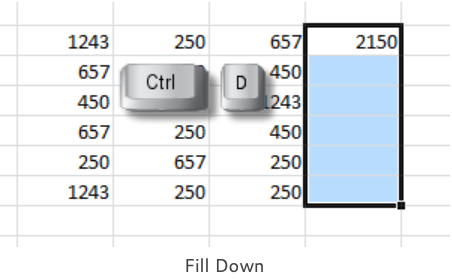
Ctrl+D and Ctrl+R  Fill Down and Fill Right

Fill formulas or data down the column by selecting down with the SHIFT and Down arrow key. Then Ctrl+D fills down the selection. Ctrl+R to fill across to the right.

fill down

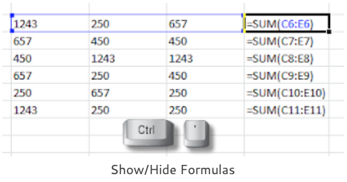
Ctrl+`  Show/Hide Formulas

You can’t check that you’ve got your formulas entered correctly if you can’t see them.

Switch between displaying the returned results of your formulas and the actual formula itself by pressing Ctrl+` (that’s  usually the key under the ESC key in the top left hand corner of the keyboard)

show hide formulas

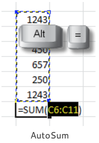
ALT+=  AutoSum

Instead of clicking the AutoSum control every five minutes ALT+= enters a sum formula into the active cell. But it only does SUM and does not give you a choice of other functions.

See my article AutoSum Revisited for a few ideas on getting the best out of AutoSum.

autosum shortcut

Ctrl+ENTER  Range Entry

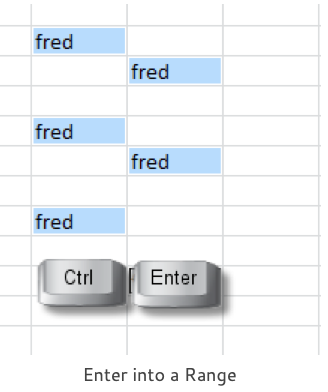
Pressing the ENTER key makes an entry into your current active cell. Ctrl+ENTER makes an entry into every single cell in your current selection. Make the selection, type in your entry and then press Ctrl+ENTER.

Constants (text or numbers) and formulas can be entered into a range in a single step. Formulas give you a relative reference for each cell, so if you get the first one right then all the others will adjust accordingly.

To enter data into a discontinuous range, make a multiple selection first. Select a cell or a range of cells then hold down the Ctrl key as you add to your selection by clicking on other cells or ranges.

enter into range

ALT+ENTER  Insert New Line

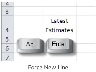
Rather than wrapping the text in the cell whenever you want to force a new line press ALT+ENTER.

This is very handy for creating Excel source data for Tables or Pivot Tables where you maybe need to have multiple lines of descriptive text for a heading but retain the integrity of the single physical header row.

force new line

F4  Absolute Reference and Repeat

When you need Absolute References (dollar signs) in your formulas press F4. Succeeding presses of the F4 key return all the permutations of absolute and relative reference: $A$1, A$1, $A1, A1.

To make a single cell reference in your formula absolute, click somewhere on the reference then press F4. For a range reference or a series of references, drag across the references first before pressing F4.

F4 has a double life, when you are in Ready mode (i.e. not editing your formulas) F4means Repeat. Say you have the tedious job of going through a worksheet and deleting some of the rows, delete the first one as you usually do and then select the next row to be deleted and press F4 to repeat the row deletion.

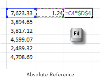
absolute references

F11  Chart

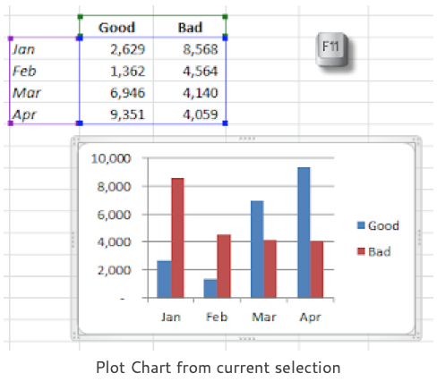
Pressing F11 plots a default chart on a separate chart sheet based on your current cell selection. Press ALT+F11 for an embedded chart on the active sheet. Excel will automatically execute a current region selection if you start with a single cell selected in your chart data range. To plot discontinuous ranges, make a multiple selection using your Ctrl key before pressing F11.
plot chart

Related Courses

Microsoft Excel Intermediate – Link

Microsoft Excel Advanced – Link

Excel Sort by Last Name

Excel Sort by Last Name

Table of Contents

sort by last name

Excel Sorting By Last Name

You have a list of names in your Excel spreadsheet with both the first and the last names in the same cell and you want to sort your list alphabetically by the last name. Not too much to ask, is it?

The bad news is Excel sorts on the entire entry in the cell reading from the left hand side and you can not specify any particular element of your text to provide the sort order. I know that’s what you want but you just can’t have it. Sorry.
Isolating the Last Names

The only way to do this is to get the last names into a separate column and then base your sort on that column and not on the existing names. Make sure that the sorting column is right next to one of the existing columns in your worksheet so that Excel captures it as part of your list. You can always hide your sorting column. 
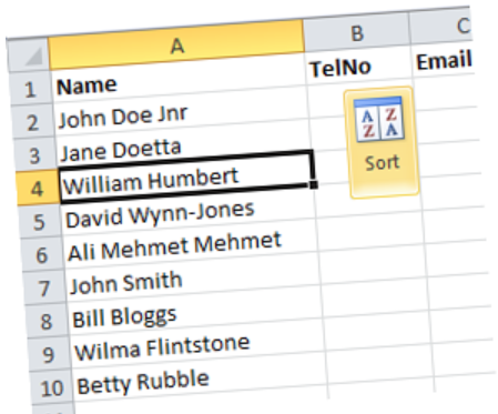
There are several methods of isolating the last names. In this article we shall be discussing Flash Fill, Text to Columns, Find and Replace and Formulas. To make your life easy, try to make your text as regular as possible as most of these processes are about finding a space in the middle of a bit of text. Any double-barrelled names like Ann Marie, Jean Paul or Wynn Jones will be much easier to process if you substitute the space with a dash, like this: Ann-Marie, Jean-Paul or Wynn-Jones.

Using Flash Fill

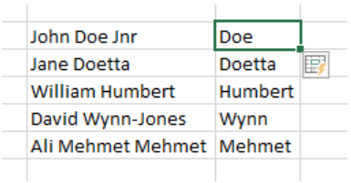
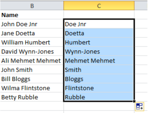
What could be easier, type in a few suggestions (I did Doe and Doetta) and then shoot over to the Data tab and click the Flash Fill control which you should be able to find in the Data Tools group. To be fussy, I could say that I really wanted to have Wynn-Jones instead of Wynn so I should have included one as an example but it’s only for sorting so I’m happy.

flash fill results

What’s your problem? You’re looking at your Data tab and you don’t have a Flash Fill control? That’s because it’s new with Excel 2013.

That’s the problem with this method; you need the software. You either have to buy a new copy of Excel or check out the rental version on Office 365.

Flash Fill is far and away the best method for this exercise and I would throughly recommend it as the program is so good at picking out patterns from your examples. The only drawback is that you would have to repeat the exercise whenever you added new names to the list. It’s worth buying a new copy of Excel just for Flash Fill.

flash fill control

Using Text to Columns

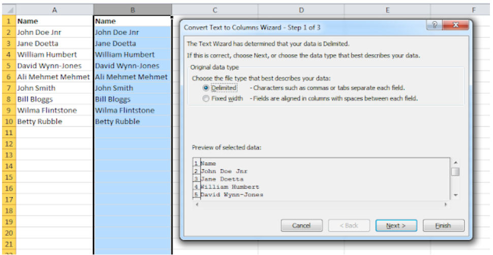
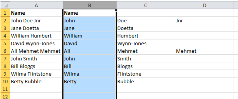
Text to Columns is where you can use the space between the first and last names as a “delimiter” and have Excel generate two columns of data; one with the first names and the other with the last names. You delete the first names column and keep the last names as your sort column. There will be issues with titles, middle names and initials etc.
text to columns step1

This is Step 1 of the Text to Columns Wizard and here you just need to specify that you are processing Delimited data and then click the Next button to move on to Step 2.

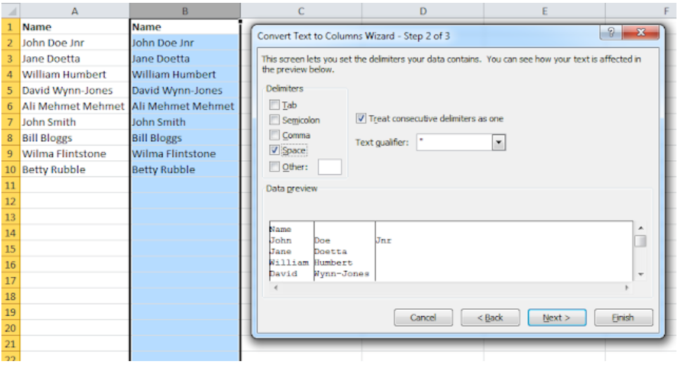
text to columns step2

Step 2 is where you specify the Delimiter; clear the Tab check box and click the check box for Space then examine the Data preview. As you can see, it’s not perfect as every space character has been used as a separator but it has done the bulk of the work so click the Finish button.

text to columns results

Here’s the resulting text, it’s been chopped-up (or parsed) into separate fragments based on wherever a space character was found in the original text. There’s still a bit of work to do as you need to delete the unwanted columns. It’s always a good idea to insert a few extra blank columns into your worksheet before using Text to Columns as this will avoid your accidentally over-writing any existing data. 

Using Find and Replace

Again, this is all about using the spaces as separators and employs two passes of Find and Replace in combination with wildcards. This is definitely one for all the Find and Replace fans, I am constantly amazed at how creative and ingenious some people can be with Find and Replace.
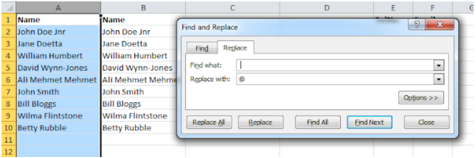
find and replace1

Click the column letter at the top of one of your columns where you have the names and then replace every space with an arbitrary character, in this case an @ sign. You can use any character you like, just make sure that it’s a character that would not be found in any of the names. Type a space into the Find what box and an @ sign into the Replace with box then click Replace All. Now all the names look something like this: Bill@Bloggs, John@Smith etc.

find and replace2

The next job is to strip out all the text up and including the last @ sign by replacing it with nothing which will then leave the last text element which is, of course, the last name. Type the following expression into the Find what box, ?*@ and leave the Replace with box empty. Click the Replace All button and you are left with the last names.

The wildcard characters used here are the question mark, ? which means “Find any type of character” and the asterisk,* which means “Find everything”. Therefore ?*@ means “Find everything leading up to and including the last @ sign”.

Using Formulas

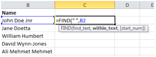
And then there are the Excel fans who would not dream of using Find and Replace because, for them, everything is done with formulas and functions for they can not be parted from their commas and brackets. The formula solution uses Text functions and is quite complex but it is constructed in stages; use the FIND or SEARCH function to read the text from the left hand side to find the position of the first space character. Then use the RIGHT function to extract the text after the space.
formula uses FIND function

This is the first step, locating the first space in the first cell:

=FIND(” “,B2)

This formula gives the result of 5, the first space is located at character index 5, after the first four characters, “John”. The FIND function is case-sensitive which does not matter if you are finding a space but it could be an issue for some other characters, in which case you should use the SEARCH function which is not case-sensitive.

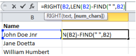
The next job is to extract the text from the right hand side up to, but not including, the space character which has now been located. Of course, the names are of varying length so you need to calculate how many characters in from the right hand side for which you need the LEN function. So the LEN of the cell minus the FIND value gives the number of characters required.

finished formula
Here’s the finished formula:

=RIGHT(B2,LEN(B2)-FIND(” “,B2))
 
Be careful with the commas and the brackets if you are hand typing or click the Insert Function (fx) button and let Excel do them for you.

The final job is to copy the formula down the column and extract all the last names.

You can leave the formulas in the cells as it will not affect the sorting and it will make any additional records much easier to process as you can just copy the existing formulas.

A final thought, why didn’t we have two columns in the first place? Then we wouldn’t have to have Excel sort by last name. The moral of the story is to store things like first names and last names in separate columns.

copy down the formula

Related Courses

Microsoft Excel Intermediate – Link

Microsoft Excel Advanced – Link

Excel Dollar Signs

Excel Dollar Signs

Table of Contents

excel F4 key

Excel Absolute References, the Dollar sign $ and the F4 key

Excel Dollar Signs or, to be correct, Absolute References are one of those things that you really need to know about if you want to be successful with your Excel formulas. And it’s good idea to know about the F4 shortcut key.

Way back in the last century we always used to say that if you didn’t know your function keys then you weren’t being serious. Thankfully, those days have passed but you still need to know the F4 key for working with Excel formulas. The F4 key will repeat the last command or keystroke when you’re working in Word, Excel or PowerPoint. However, it’s primary use in Excel is for inserting the dollar signs ($) for Absolute cell references in your Excel formulas.

You may have seen cell references in formulas surrounded by ‘$’ signs, for example $D$3:$D$10, and wondered what’s that all about?  The ‘$’ before the column or row reference fixes the reference so that it does not change when it’s copied. You either have to type in the $ signs or press the F4 key. Be careful with the F4 key on your laptop, if it does not seem to work properly then press Fn and F4 together. Press CMD+T if you’re working with Excel for Mac.

Using Absolute References in Formulas

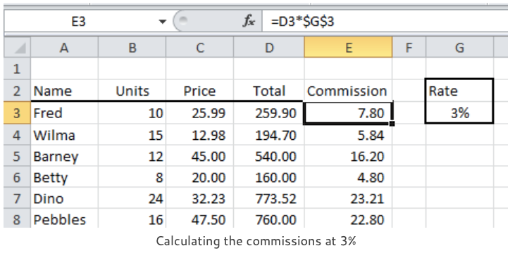
calculating the commissions at 3%

For example, looking at the table above we have a Commission Rate of 3% in cell G3. In column E we want to calculate the commission as Total x Rate @ 3%. We could simply enter the formula as =D3*3% and copy it down column E, but then that gives us two major problems to deal with:

  1. We can’t easily see what the commission rate is without looking in the formula bar. We could include it in the column heading as “Commission @ 3%”, but that makes the heading too wide and if I should change the rate then I will have to remember to go back and change the heading as well.
  2. If I do change the rate then I need to change the formula and copy it down the column again. Doing this once would be acceptable but not if I need to do it regularly and what if other formulas are using the commission rate? It would be so much easier just to have the commission rate in a single cell.

In the formula for the commission calculation, the commission rate of 3% is entered into cell G3 and then the G3 reference is used in our formulas like this, =D3*$G$3. The reference is absolute, meaning that it never changes wherever the formula is copied.

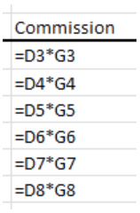
relative references

Let’s look at what happens if we don’t use an absolute reference. If we entered in cell E3 the formula =D3*G3 we would get the correct answer. But when we copy that formula down the rest of column E Excel updates the cell references in the formula to increase by one row as we go down. You can see this to the left where the references to D3 and G3 change to D4 and G4 etc. 

These standard cell references are known as relative references. We want the D3 reference to change but we want the G3 reference to be fixed.

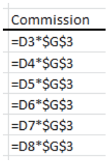
To keep the commission rate reference on cell G3 we enter the formula like this, =D3*$G$3. Then when we copy the formula down the column the column D references change but the reference to cell G3 does not.

Strictly speaking, we only needed to fix the reference to row 3 as the G column reference would not have changed but it’s usually easier just to fix the entire cell reference and have done with it. The difficult bit is to realise that you needed an absolute reference in the first place.

absolute references

Other ways to use Absolute References

  • Make a whole range of cells an absolute reference: $D$1:$F$1
  • Make only the column absolute: $D3
  • Make only the row absolute: D$3

To help you see how your formulas are behaving it’s quite a good idea if you can actually see them instead of the results of the formula. To display your formulas in the worksheet, click the Show Formulas control on the Formula Auditing group of the Formulas tab.

F4 Shortcut for entering Absolute References

The F4 key instantly enters the ‘$’ signs for you. You can do it while you’re entering your formula or you can go back and edit the original formula.
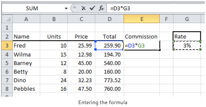
In the example below we have started to enter a formula into cell E3. We have just selected cell G3, as you can see by the marquee (“marching ants”) around the cell.

entering the formula

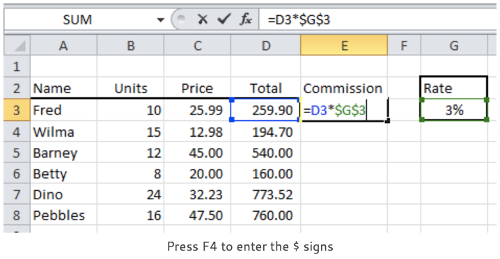
At this point, before pressing ENTER or clicking the tick to finish the formula, we can press the F4 key and Excel places the ‘$’ signs around the G3 reference. Or you can go back to a cell at any time. Press the F2 key to edit the formula if you are feeling old-fashioned, or just double-click the cell. Click anywhere in the cell reference and press F4 to insert the $ signs.

press F4 to enter the $ signs
fixing a range

If you want to fix a range reference you have to highlight the cell range in the formula before pressing F4. If you keep pressing F4 Excel iterates through all the permutations of absolute and relative reference:

  • With the first press of F4 you get $G$3. Column and row absolute.
  • With the second press of F4 you get G$3. Column relative and row absolute.
  • With the third press of F4 you get $G3. Column absolute and row relative.
  • With the fourth press of F4 you get G3. Column and row relative.

Mixed Relative and Absolute references

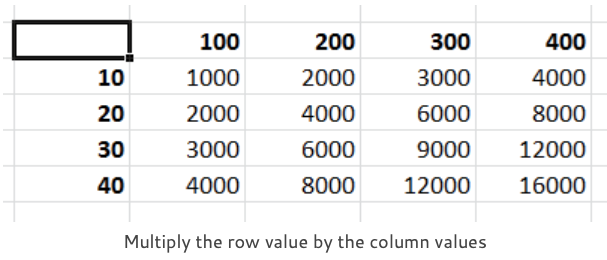
Whilst it usually easier to fix the entire reference there are times when you must have a mixed reference, where only the row or the column is fixed, in order to make your formulas work. In the worksheet example below we are multiplying all the hundreds values in the top row against all the tens values in the first column of the table. The first formula multiplies the 10 by the 100, =B3*C2.

multiply the row value by the column values

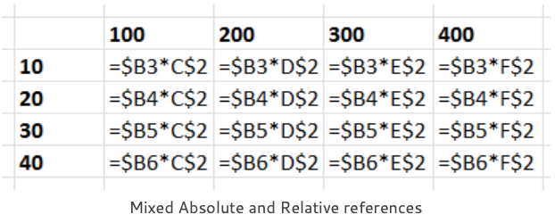
As the formula is copied across and down we need the row reference for the hundreds values to be fixed and the column reference for the column reference for the tens values to be fixed. But the rest of the formula must be relative so that it works correctly when it is copied.

mixed absolute and relative references

Usually I try to work out this type of formula logically before I start. And usually it goes wrong so I just resort to experimentation until I get it right. It only takes me an hour or so. Best of luck with your Excel Dollar Signs!

Related Courses

Microsoft Excel Intermediate – Link

Microsoft Excel Advanced – Link

Microsoft Excel Flash Fill

Microsoft Excel Flash Fill

Table of Contents

Microsoft excel flash fill

Excel – Flash Fill

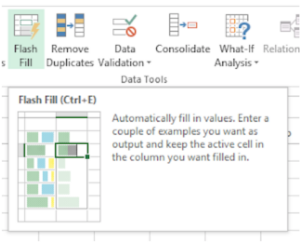
flash fill control

Sometimes, half the problem is getting data into Excel so that you can work on it. You run a query on a database and get a mishmash of poorly formatted data. Hundreds of rows full of data you don’t want mixed with the few odd bits that you do. Been there? This is where you need Excel 2013’s Flash Fill to come to your rescue.

To make sense of your data, type in a few row’s as an example of what you need and then click Flash Fill to do the rest of the work for you. Excel applies the lessons learnt from your examples to the rest of the data, with all the columns below filling with the correctly formatted data. No complicated formulas and no macros required. And no retyping!

You can extract simple patterns from your data, for example extract the first name from a full name or you can extract multiple patterns. For example, you can get the date, the business name and the amount from a credit card statement. All by typing a couple of examples for Excel to use as a template.

The Microsoft Excel Flash Fill control is on the Home tab of the ribbon in the Fill group. It is also found in the Data Tools group on the Data tab. And, of course, you can add it to your Quick Access Toolbar if you find yourself using it frequently.

flash fill in data tab

Flash Fill Example

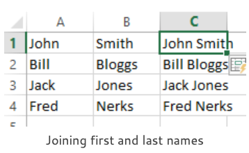
join first and last names

Here’s a simple exercise; joining first and last names together in the same cell. Type the example “John Smith” into column C and then click Flash Fill to do the rest.

That’s an easy one. If you know Excel formulas you could do that as
=A1&B1 or =CONCATENATE(A1, B1)

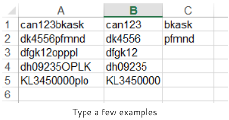
Let’s try the Microsoft Excel Flash Fill challenge, a really hard one. In this exercise we need to parse the data in the first column so that a series of numbers appearing after a series of letters is identified and the text after the series of numbers is extracted.
 
I am getting a headache just thinking about how I would do this one with a formula…
type a few examples
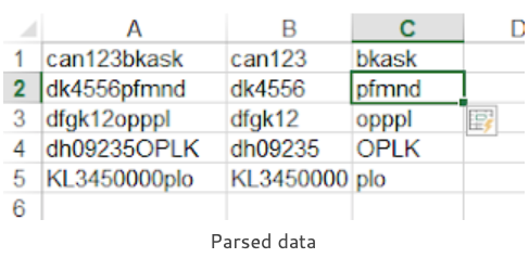
parsed data

Begone with your complicated formulas and Text-to-Columns routines. Type-in a couple of examples and let Flash Fill take over. The results are seriously impressive.

Try doing that with a formula. I’ve still got that headache.

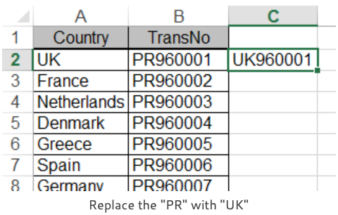
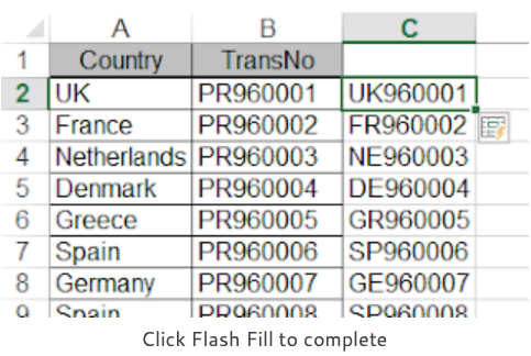
Let’s try one more; here we need to remove the two-letter prefix “PR” from the front of the entries in column B and replace it with the first
two letters of the country entered in column A. As capital letters.
 
Enter the first item in column C to set the pattern and then click Flash Fill to do the rest. Fantastic!
replace the PR with UK
click flash fill to complete
Well, I think that we could have done this one using the LEFT, RIGHT and UPPER functions to extract and convert the relevant data. Then concatenated the results to produce the new transaction code.
 
But the point is, we don’t have to do that sort of thing any more and I for one will not miss it at all. This is the kind of machine learning and artificial intelligence that we all appreciate. 

Related Courses

View Excel Training Courses – Link

Switching Excel Columns to Rows

Switching Excel Columns to Rows

Table of Contents

Switching_Excel_Columns_to_Rows

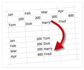
Switching Excel Columns to Rows. You should really call this Transposition if you want to impress. Excel data can be rearranged from columns to rows and vice versa. You can transpose as many rows or columns as you like all in one go. You need to decide whether you want to do the transposition just once or have the transposed data update to reflect any changes made to the original.

Switching_Excel_Columns_to_Rows

Static Transposition

Static transposition is where the data is rearranged just once and it’s really easy to do. However, dynamic transposition, where you have two sets of Excel data; one arranged in columns and the other in rows, is much more difficult and involves your entering an array formula.

If you know how to Copy and Paste then you’ll find static transposition a breeze. The copy bit is as normal but there is a variation to the paste bit. Select the original range of cells and Copy them. Then click a blank cell that is away from the original range and Transpose; there is no need to select the entire range for the transposition, a single cell is all you need.

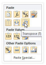
Excel_Paste_Menu

Finding the Transpose command depends on which version of Excel you are using. If you have a modern version of Excel with the fancy ribbons then you should be able to find Transpose in the Paste control on the Home tab or in the shortcut menu when you right-click.

Should you have one of the good old fashioned versions with the drop-down menus then look for Paste Special which is found in the Edit menu. Failing that right-click after you have done your Copy and you may very well find Paste Special in the shortcut menu.

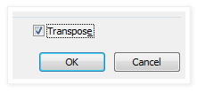
When the Paste Special dialog appears you need to find the Transpose check box, give it a click and then click the OK button. Sounds easy doesn’t it? But I often find myself staring at the screen muttering “now, where’s that Transpose thingy…”. Because it’s right down the bottom, where it always has been.

Excel_Transpose

Dynamic Transposition

In the previous example we transposed our data and ended up with two independent ranges of cells, one of which you would probably want to delete. You might want to keep both ranges and have the transposed data change when changes were made to the original. This where you need to have a formula. The most painful method would be to go through each cell, enter an equals sign and click the corresponding cell in the original range. Very tedious indeed.

A much better method would be to create an array formula using the TRANSPOSE function. Array formulas are not easy to enter and most sensible people run screaming from the room at the mere mention of them. So don’t get annoyed if this formula takes a few goes to get right. Like most Excel formulas you have to persevere and suffer for a bit until you feel confident.

Entering an Array formula

Exce Buttons

Array formulas are entered into ranges of cells in one go. They are not entered into single cells and then copied which is what we are used to. You select the range, enter the text of the formula and finally, press CTRL+SHIFT+ENTER on your keyboard to enter your formula into the selected range.

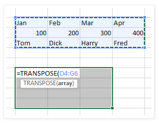
The first job is to count the number of rows and columns in the range that you wish to transpose. Then select a range of empty cells whose dimensions correspond to the inverse of the original range. For example, I want to transpose the range D4:G6, which is a range with 5 columns and 3 rows, so I select an range of 3 columns by 5 rows.

Excel_Sub_menu

Now we enter the required formula. The formula is as follows “=TRANSPOSE(D4:G6)”. Then, holding down the CTRL and SHIFT keys, press ENTER or click the Enter box in the formula bar.

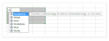
If you have a version of Excel that pops up the list of functions as you type then you can accept TRANSPOSE from the list by pressing the TAB key. Array formulas are identified in the formula bar enclosed in braces (the squiggly brackets) but you do not type in the braces when you enter the formula.

Excel_Transpose_function

Working with Array formulas

You may not change part of an array formula. If you want to delete your formula, select the entire formula first before pressing the Delete key. To edit the formula there is no need to select the whole array first but don’t forget to press CTRL+SHIFT+ENTER to accept the edit.

The Excel shortcut key to select the current array is CTRL+/ (front slash). If you have a huge transposition just click one cell and then the short cut key will select the rest of it for you.

When you are counting the number of columns or rows in a large range it is all too easy to lose count and very frustrating when you have to start over again. “One, two, three, four… ” Such fun. Use the Excel functions ROWS or COLUMNS to calculate the dimensions of large ranges rather than count them. For example, the formula =ROWS(A1:D50) returns the value of 50.

Excel Transpose Example
Transpose_Example 2

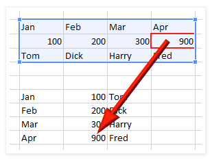
Transposition formulas are not the easiest of formulas to get right but, like all formulas, once they are done they will look after themselves and update automatically.

Any changes made to the original range are immediately reflected in the transposition.

Related Courses

Microsoft Excel Intermediate – Link

Microsoft Excel Advanced – Link

Training Courses

If you’ve still got that “I just don’t know what I’m doing” feeling then you might like to arrange an Excel training course for yourself or with some of your colleagues. It’s really easy to book one of our courses and they’re great value for money. See our website for full details.
Switching Excel Columns to Rows by Mouse Training London

Microsoft Project 2019

Microsoft Project 2019 What's New

Table of Contents

icons8-microsoft-project-100

A fresh new experience

Microsoft Project 2019 offers a redesigned user experience that is both simple and intuitive. Your teams can quickly add new members and set up tasks, then easily switch between grids, boards or timeline (Gantt) charts to track progress. Because Project is part of the Microsoft 365 family, project teams can save time and do more with built-in connections to familiar apps like Microsoft Teams and Office.

Project 2019
Project 2019 b

Collaboration made easy

Microsoft Project 2019 is designed to do much more than just track progress. Project works with Teams to support collaboration and makes it easy to manage all aspects of a team project, including file sharing, chats, meetings and much more. Team members in scattered locations can even edit tasks simultaneously. This way, they can get more done together, no matter where they are. To help teams stay on track, Project offers an automated scheduling engine based on effort, duration, and resources.

Project 2019 c

Project with Teams

Project with Teams

Insights at your fingertips

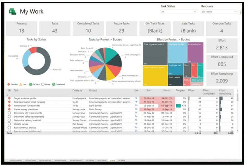
The new Microsoft Project 2019 provides greater visibility into your projects and powerful tools to help you anticipate future needs. Create stunning interactive dashboards in Power BI, so you can visualize every aspect of each project at a glance. Get the big picture view of all your projects across your organization with the visual, interactive Roadmap feature.

Project 2019

Extensible platform

Project is built on the Microsoft Power Platform. This enables you to connect to the apps and services you already use and also to create custom desktop and mobile experiences to meet the specific needs of every project team. Easy to use tools make it simple to create automated workflow processes that streamlines compliance and increases efficiency. Do all this and more with the confidence that comes with knowing you are building on the powerful security and compliance capabilities of Azure—the world’s most trusted enterprise cloud.

Hints and Tips

Office 365 Groups

Microsoft Office 365 Groups

Table of Contents

office 365 groups

What are Office 365 Groups?

Microsoft Office 365 Groups lets you to collaborate with your teammates when writing documents, creating spreadsheets, working on project plans, scheduling meetings and sending email. Office 365 release 2019 is a new service available to 365 and 2019 Outlook users.

Groups lets you choose a set of people that you wish to collaborate with and also set up a collection of resources for them to share. For example; a shared Outlook inbox, a shared calendar or a document library for collaborating on files.

You don’t have to manually assign permissions to all these resources because you automatically give the required permissions when you add members to the group. Any member of the group can use the tools that your group provides. Groups are the new and improved method for what we used to do using distribution lists or shared mailboxes.

Office 365 Groups can be created from:

  • Outlook on the web
  • Outlook Mobile
  • SharePoint
  • Planner
  • Teams

Which tool you choose to start from depends on what kind of group you’re working with. For example, most will tend to start from Outlook when creating a Group organised around email and calendar. If the Group is for company wide communication you would tend to start with Yammer. For chat-based collaboration start your Group from Microsoft Teams.

Creating Groups

When creating a group where you can collaborate with your teammates you need to decide if you want it to be a private group or a public group. Content in a public group can be seen by anybody in your organisation and anybody in your organisation is able to join the group. Whereas content in a private group can only be seen by the members of the group and people who want to join a private group have to be approved by a group owner.

Neither public groups nor private groups can be seen or accessed by people outside of your organisation unless those people have been specifically invited as guests.

Adding guests to Office 365 Groups

Guest access 

Office 365 Groups lets you and your team collaborate with people from outside your organisation by granting them access to group conversations, files, calendar invitations and the group notebook. Access can be granted to a guest—for example, a partner, vendor, supplier, or consultant—by any group owner.

How it works?

People using Office 365 Groups can use Outlook on the web or Outlook for Windows to add and manage guests in their Office 365 groups. Guests can have any email address, and their email account can be a work, personal, or school account.

Note: Guest access is set up by the IT administrator.

  1. A group owner adds a guest to the group or a guest is nominated by a group member. The group owner approves the nominees.
  2. The group owner is informed of which content and resources the guest can access within the group. A combination of text and icons gives all group members a clear indication of guest participation.
  3. The guest receives a welcome email and can participate in group conversations, receive and respond to calendar invitations, and access the group files.
  4. Guests can leave the group at any time via a link in the footer of all group email messages and calendar invitations.

Admins can manage guests and their access to Office 365 group resources using PowerShell. See Manage guest access in Office 365 Groups for instructions.


When a guest is invited to join a group, they receive a welcome email message that includes a little information about the group and what they can expect now that they’re a member. The message also includes a set of links to help them get started and connect to group resources.
OutlookGroups

The guest member’s interactions all occur through their email inbox. They can’t access the group site but can receive calendar invitations, participate in email conversations and, if the admin has turned on the setting, they can open shared files using a link or attachment.

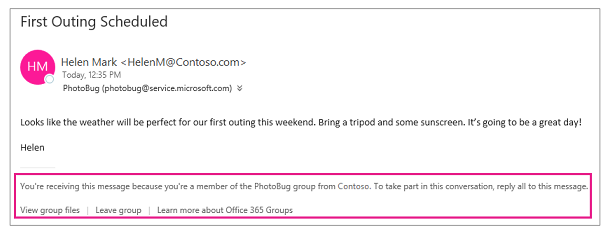
All group email messages and calendar invitations the guest receives will include a reminder to use Reply all in responses to the group, along with links to view group files and leave the group.

FirstOutingScheduled

The following table summarises what guests can and can’t do.

GuestCanAndCantDo