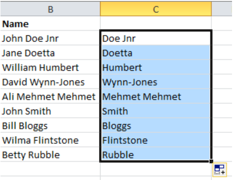
Excel Sort by Last Name
Table of Contents
Excel Sorting By Last Name
You have a list of names in your Excel spreadsheet with both the first and the last names in the same cell and you want to sort your list alphabetically by the last name. Not too much to ask, is it?
The bad news is Excel sorts on the entire entry in the cell reading from the left hand side and you can not specify any particular element of your text to provide the sort order. I know that’s what you want but you just can’t have it. Sorry.
Isolating the Last Names
The only way to do this is to get the last names into a separate column and then base your sort on that column and not on the existing names. Make sure that the sorting column is right next to one of the existing columns in your worksheet so that Excel captures it as part of your list. You can always hide your sorting column.
There are several methods of isolating the last names. In this article we shall be discussing Flash Fill, Text to Columns, Find and Replace and Formulas. To make your life easy, try to make your text as regular as possible as most of these processes are about finding a space in the middle of a bit of text. Any double-barrelled names like Ann Marie, Jean Paul or Wynn Jones will be much easier to process if you substitute the space with a dash, like this: Ann-Marie, Jean-Paul or Wynn-Jones.
Using Flash Fill
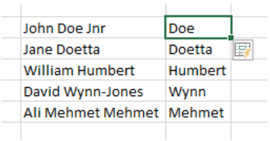
What could be easier, type in a few suggestions (I did Doe and Doetta) and then shoot over to the Data tab and click the Flash Fill control which you should be able to find in the Data Tools group. To be fussy, I could say that I really wanted to have Wynn-Jones instead of Wynn so I should have included one as an example but it’s only for sorting so I’m happy.
What’s your problem? You’re looking at your Data tab and you don’t have a Flash Fill control? That’s because it’s new with Excel 2013.
That’s the problem with this method; you need the software. You either have to buy a new copy of Excel or check out the rental version on Office 365.
Flash Fill is far and away the best method for this exercise and I would throughly recommend it as the program is so good at picking out patterns from your examples. The only drawback is that you would have to repeat the exercise whenever you added new names to the list. It’s worth buying a new copy of Excel just for Flash Fill.

Using Text to Columns
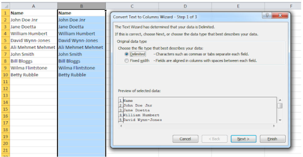
This is Step 1 of the Text to Columns Wizard and here you just need to specify that you are processing Delimited data and then click the Next button to move on to Step 2.
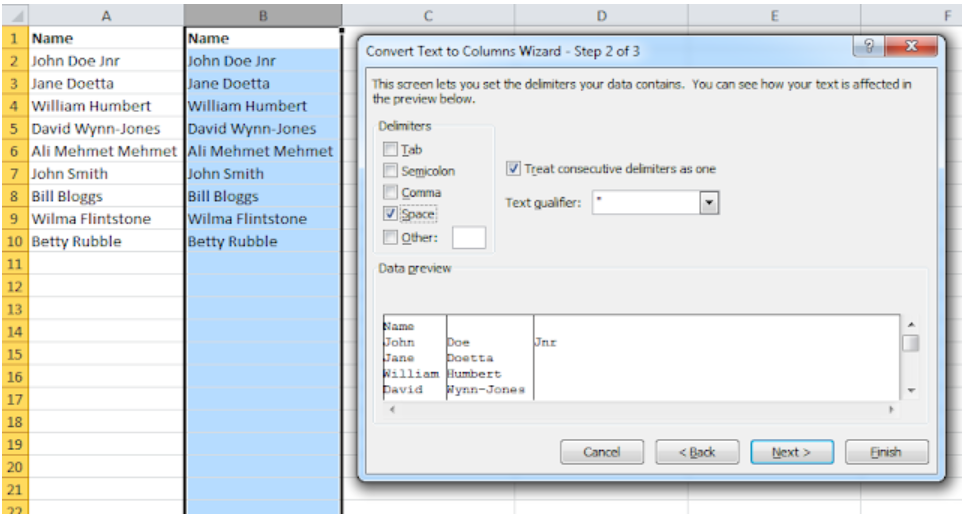
Step 2 is where you specify the Delimiter; clear the Tab check box and click the check box for Space then examine the Data preview. As you can see, it’s not perfect as every space character has been used as a separator but it has done the bulk of the work so click the Finish button.
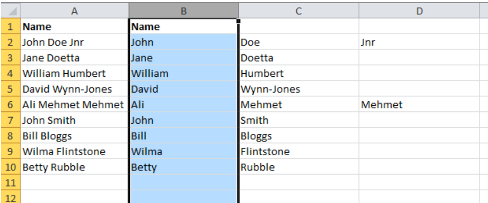
Here’s the resulting text, it’s been chopped-up (or parsed) into separate fragments based on wherever a space character was found in the original text. There’s still a bit of work to do as you need to delete the unwanted columns. It’s always a good idea to insert a few extra blank columns into your worksheet before using Text to Columns as this will avoid your accidentally over-writing any existing data.
Using Find and Replace
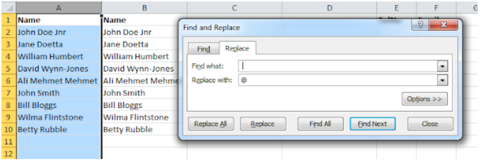
Click the column letter at the top of one of your columns where you have the names and then replace every space with an arbitrary character, in this case an @ sign. You can use any character you like, just make sure that it’s a character that would not be found in any of the names. Type a space into the Find what box and an @ sign into the Replace with box then click Replace All. Now all the names look something like this: Bill@Bloggs, John@Smith etc.

The next job is to strip out all the text up and including the last @ sign by replacing it with nothing which will then leave the last text element which is, of course, the last name. Type the following expression into the Find what box, ?*@ and leave the Replace with box empty. Click the Replace All button and you are left with the last names.
The wildcard characters used here are the question mark, ? which means “Find any type of character” and the asterisk,* which means “Find everything”. Therefore ?*@ means “Find everything leading up to and including the last @ sign”.
Using Formulas
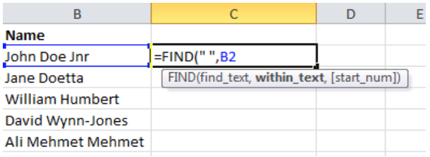
This is the first step, locating the first space in the first cell:
=FIND(” “,B2)
This formula gives the result of 5, the first space is located at character index 5, after the first four characters, “John”. The FIND function is case-sensitive which does not matter if you are finding a space but it could be an issue for some other characters, in which case you should use the SEARCH function which is not case-sensitive.
The next job is to extract the text from the right hand side up to, but not including, the space character which has now been located. Of course, the names are of varying length so you need to calculate how many characters in from the right hand side for which you need the LEN function. So the LEN of the cell minus the FIND value gives the number of characters required.
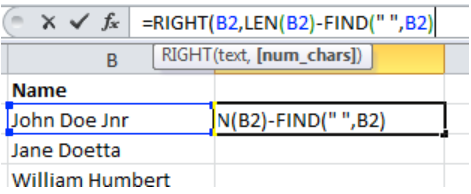
The final job is to copy the formula down the column and extract all the last names.
You can leave the formulas in the cells as it will not affect the sorting and it will make any additional records much easier to process as you can just copy the existing formulas.
A final thought, why didn’t we have two columns in the first place? Then we wouldn’t have to have Excel sort by last name. The moral of the story is to store things like first names and last names in separate columns.
