Excel Make Pivot Tables Refresh Automatically
Table of Contents

Excel – Make Pivot Tables Refresh Automatically. Excel Pivot Tables do not automatically update when their source data is changed. Unlike formulas they have to be refreshed. That’s no problem if you can remember to do it, but it’s all too easy to forget.
To make your Pivot Tables refresh automatically you need a Macro to do the refreshing and an Event to trigger the macro. You record a macro of your refreshing the Pivot Table and then you copy the recorded code and paste it into one of the worksheet’s events. This seems quite an involved process the first time you do it. But it gets easier every time you repeat it as it is just copying and pasting from one workspace to another.

Recording the Macro
Firstly, make the recording. Select a cell in your Pivot Table and then click the Record Macro control in the Macros group at the extreme right of the View tab.
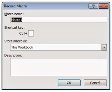
Make sure that the Store macro in: setting is This Workbook and click the OK button. Now you have to record your refreshing the Pivot Table; just right-click the active cell and choose Refresh from the shortcut menu. The recording is now completed and you have to turn off the macro recorder by clicking the Stop Recording control in the Macros group on the View tab.

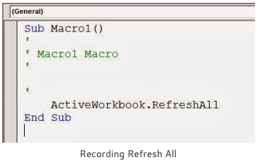
The next job is to find the recorded code and copy the instruction that refreshes your Pivot Table. Click the View Macros control in the Macros group on the View tab, select your recorded macro from the list and then click the Edit button on the right hand side. You will now see your recording displayed in the Visual Basic Editor, it should look something like this:

Using an Event to trigger the Macro

Next, you need to find the Events for the worksheet where your Pivot Table is located. Every Excel worksheet has a collection of event-driven macros which trigger automatically whenever a particular event occurs. For example, the Selection Change event is triggered whenever you click a cell on the worksheet. We are going to use the Activate event to make our Pivot Table refresh.
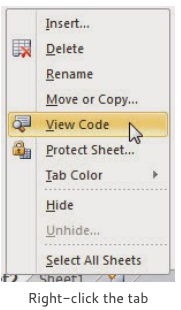
Right-click the worksheet tab and choose View Code from the shortcut menu. You are returned to the Visual Basic Editor once again but this time the screen looks blank. Don’t let that put you off, looking at the top of the active window you will see two drop-down lists.

Go to the Object list on the left and select the Worksheet object and then choose a suitable event from the Procedure list on the right.

All objects have default events and these usually appear in the window automatically, ignore them and scroll up the list to select the Activate event. Paste your recording into the event procedure so that it looks like this:

Return to the Excel workspace by clicking an Excel icon or by pressing ALT+F11, select another worksheet in the workbook and then return to the original worksheet where the Pivot Table is stored. This triggers the event and you will see that the tables are automatically refreshed. The best test is to change something in your source data and then see if your Pivot Table updates to reflect the change.
Using your Macro Again
If you have several Pivot Tables that need to be refreshed then it is quite in order to list the various Pivot Tables one after the other in your macro but it is probably best if you recorded Refresh All in which case the initial recording would like the illustration on the right.
Saving your file
When your Excel workbook file contains macros remember to save the file in the Excel Macro-Enabled Workbook format.

Make Excel Pivot Tables Refresh Automatically Summary
I hope you managed to follow all of this and you get a successful result. It’s only a macro recording and a copy and paste but well worth the effort as now you will never have to remember to refresh your Pivot Tables.
If you also need to automatically update the definition of the source data range before refreshing the data, see the article Excel- Automatically change the Pivot Table source data range.