Switching Excel Columns to Rows
Table of Contents
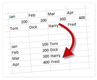
Switching Excel Columns to Rows. You should really call this Transposition if you want to impress. Excel data can be rearranged from columns to rows and vice versa. You can transpose as many rows or columns as you like all in one go. You need to decide whether you want to do the transposition just once or have the transposed data update to reflect any changes made to the original.

Static Transposition
Static transposition is where the data is rearranged just once and it’s really easy to do. However, dynamic transposition, where you have two sets of Excel data; one arranged in columns and the other in rows, is much more difficult and involves your entering an array formula.
If you know how to Copy and Paste then you’ll find static transposition a breeze. The copy bit is as normal but there is a variation to the paste bit. Select the original range of cells and Copy them. Then click a blank cell that is away from the original range and Transpose; there is no need to select the entire range for the transposition, a single cell is all you need.
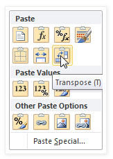
Finding the Transpose command depends on which version of Excel you are using. If you have a modern version of Excel with the fancy ribbons then you should be able to find Transpose in the Paste control on the Home tab or in the shortcut menu when you right-click.
Should you have one of the good old fashioned versions with the drop-down menus then look for Paste Special which is found in the Edit menu. Failing that right-click after you have done your Copy and you may very well find Paste Special in the shortcut menu.
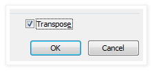
When the Paste Special dialog appears you need to find the Transpose check box, give it a click and then click the OK button. Sounds easy doesn’t it? But I often find myself staring at the screen muttering “now, where’s that Transpose thingy…”. Because it’s right down the bottom, where it always has been.
Dynamic Transposition
In the previous example we transposed our data and ended up with two independent ranges of cells, one of which you would probably want to delete. You might want to keep both ranges and have the transposed data change when changes were made to the original. This where you need to have a formula. The most painful method would be to go through each cell, enter an equals sign and click the corresponding cell in the original range. Very tedious indeed.
A much better method would be to create an array formula using the TRANSPOSE function. Array formulas are not easy to enter and most sensible people run screaming from the room at the mere mention of them. So don’t get annoyed if this formula takes a few goes to get right. Like most Excel formulas you have to persevere and suffer for a bit until you feel confident.
Entering an Array formula

Array formulas are entered into ranges of cells in one go. They are not entered into single cells and then copied which is what we are used to. You select the range, enter the text of the formula and finally, press CTRL+SHIFT+ENTER on your keyboard to enter your formula into the selected range.
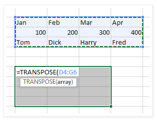
The first job is to count the number of rows and columns in the range that you wish to transpose. Then select a range of empty cells whose dimensions correspond to the inverse of the original range. For example, I want to transpose the range D4:G6, which is a range with 5 columns and 3 rows, so I select an range of 3 columns by 5 rows.
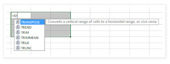
Now we enter the required formula. The formula is as follows “=TRANSPOSE(D4:G6)”. Then, holding down the CTRL and SHIFT keys, press ENTER or click the Enter box in the formula bar.
If you have a version of Excel that pops up the list of functions as you type then you can accept TRANSPOSE from the list by pressing the TAB key. Array formulas are identified in the formula bar enclosed in braces (the squiggly brackets) but you do not type in the braces when you enter the formula.

Working with Array formulas
You may not change part of an array formula. If you want to delete your formula, select the entire formula first before pressing the Delete key. To edit the formula there is no need to select the whole array first but don’t forget to press CTRL+SHIFT+ENTER to accept the edit.
The Excel shortcut key to select the current array is CTRL+/ (front slash). If you have a huge transposition just click one cell and then the short cut key will select the rest of it for you.
When you are counting the number of columns or rows in a large range it is all too easy to lose count and very frustrating when you have to start over again. “One, two, three, four… ” Such fun. Use the Excel functions ROWS or COLUMNS to calculate the dimensions of large ranges rather than count them. For example, the formula =ROWS(A1:D50) returns the value of 50.
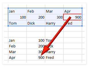
Transposition formulas are not the easiest of formulas to get right but, like all formulas, once they are done they will look after themselves and update automatically.
Any changes made to the original range are immediately reflected in the transposition.